Revisiting CAST: World-Frame Motion Model

Last year I published my first paper with SPARK lab, proposing a Certifiably optimal Algorithm for object Shape estimation and pose Tracking over time (CAST). The tracking problem is a fundamentally non-convex optimization problem due to the presence of rotations. Despite this, we showed that reformulating the problem as a quadratically-constrained quadratic program led to a tight convex relaxation in many real-world scenarios. It's part of a line of research that shows many NP-hard problems are often polynomial time in common robotics applications.

The post revists a key part of CAST: the constant-twist motion model for between-frame motion. I do not go into great detail on the algorithm or relaxation here; please refer to the paper.

Edit (June 2025): CAST-W has been fleshed out in my Master's thesis, also available below.

Part 1: The Motion Model

A key idea in object tracking is to enforce physically plausable object motion across frames. We impose a motion model, which essentially enforces continuity of motion (and perhaps biases that motion from knowledge of the object dynamics). For example, car tracking algorithms often use a constant velocity and turn rate model. Even more common is just constant velocity or constant acceleration.

CAST uses a constant-twist motion model. This keeps the twist vector (body frame velocity and rotation rate) constant across frames. Visually, it models a spiral motion:

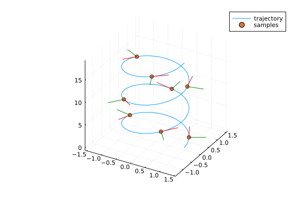
We really use a noisy version of this model: velocity $v$ is constant up to random Gaussian noise $\epsilon\sim\mathcal{N}(0,\Sigma)$, and rotation rate $\Omega$ is constant up to random Langevin noise $R_\epsilon\sim\mathcal{L}(\kappa)$. Mathematically, this is pretty simple:

The "constant-twist" part refers to updating rotations $R$ and positions $p$ in the body frame:

Constant World-Frame Velocity

The constant-twist motion model (2) works, and that alone is an interesting theoretical contribution to the space of certifially optimal algorithms. However, the bilinear constraints $R_t v_t$ are inconvenient; they prevent marginalizing out position and velocity in terms of rotation and reducing the size of the optimization problem.

As we will see, the constant world-frame velocity model does not have this issue, significantly speeding up computation. At face, the world-frame velocity model seems like an excessive simpliciation. It models straight line motion of a spinning object:

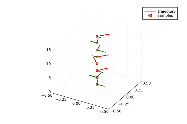
There aren't a lot of objects that move this way–most are constrained to a plane (the ground) or rotate their velocity with their orientation. However, we can add noise as in (1) which essentally represents general continuous motion:

For short time frames, this should do the job of enforcing continuous motion.

Part 2: Marginalizing Postion & Velocity

The constant world-frame velocity motion model is clearly less accurate, but it allows marginalizing out position and velocity. In short, the problem is convex holding rotations constant; the first order conditions describe the optimal $p$ and $v$ given $R$.

Let's work through a simpler version of the problem, omitting the shape vector and angular velocity terms. This is for ease of presentation; it does not fundamentally change the algebra.

The constant world-frame velocity model is the constraint $s_{t+1} = s_t + v_t$. Crucially, the position $s_t$ is only a function of $v$, not any rotations. This optimization problem is convex in $v_t$ and $s_t$ holding $R_t$ constant, so we can solve it via first-order conditions. The Lagrangian is:

Taking the derivative, we have the following equations:

Together with the equality constraint $s_{t+1} = s_t + v_t$, we have a linear system of equations:

where $A$ is composed of the (constant) coefficients of $s,v,\lambda$ in the first order conditions and equality constraint, while $b$ is the terms which do not depend on $s,v,\lambda$. In particular, $A$ is independent of $R$ and $b(R)$ is a linear function of $R$. Thus, inverting $A$ allows solving for $s$ and $v$ in closed form in terms of $R$. Plugging this in to the objective does not change the QCQP form. It only reduces the decision space, significantly speeding up computation.

Part 3: Speed

The major advantage of the world-frame velocity model is pure speed. Empirically, it runs around 5 times faster than the body-frame velocity model, depending on the number of times steps $T$ we consider. For short time steps, the performance of the more realistic body-frame velocity model is almost indistinguishable from the world-frame velocity model. I show this on the real-world drone tracking data from our paper:

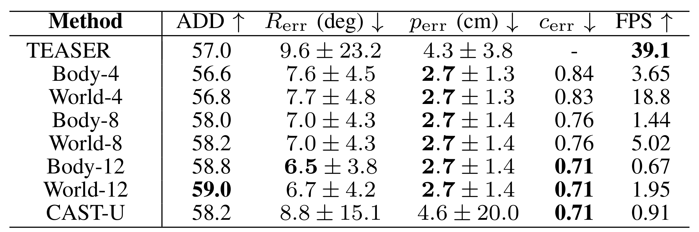
It seems like we can have our cake and eat it too: we can use a simpler model and marginalize position and velocity for significant speed improvements without sacrificing accuracy. As long as we run tracking fast enough, any first-order approximation will be reasonable and the fixed-lag will take care of large, long-term deviations from the motion model.

I don't want to completely dismiss the body-frame model. A unique part of working with convex relaxations is the art of making an informed guess about whether a relaxation is tight. From that perspective, a body-frame model is interesting because it remains tight despite the bilinear motion model. Further, we expect the body-frame model to be much more accurate as the time step between samples grows.

I want to thank Prof. Zac Manchester for suggesting we take a closer look at the world-frame model.

Code for Visuals

Constant-Twist (Body-Frame Velocity) Motion

# spiral
t = LinRange(0,6*π,1000)
Plots.plot3d(cos.(t), sin.(t), t,label="trajectory")

t2 = LinRange(0.5,5*π+2, 8)
Plots.scatter3d!(cos.(t2), sin.(t2), t2,label="samples")
Plots.quiver!(cos.(t2),sin.(t2),t2, quiver=(-0.5*sin.(t2), 0.5*cos.(t2), 0.5*ones(8)), color=:red)
Plots.quiver!(cos.(t2),sin.(t2),t2, quiver=(0.5*cos.(t2), 0.5*sin.(t2), -0.5*zeros(8)), color=:green)
# Plots.quiver!(cos.(t2),sin.(t2),t2, quiver=(-0.5*sin.(t2), 0.5*cos.(t2), -0.5*ones(8)), color=:blue)

World-Frame Velocity Motion

# straight line
t = LinRange(0,6*π,1000)
Plots.plot3d(0 .*t, 0 .*t, t, label="trajectory", ylim=[-0.5,0.5], xlim=[-0.5,0.5])

t2 = LinRange(0.5,5*π+2, 8)
Plots.scatter3d!(0 .*t2, 0 .*t2, t2,label="samples")
scale = 0.15
Plots.quiver!(0*t,0*t,t2, quiver=(-scale*sin.(t2), scale*ones(8), scale*cos.(t2)), color=:red)
Plots.quiver!(0*t,0*t,t2, quiver=( scale*cos.(t2), -scale*zeros(8), scale*sin.(t2)), color=:green)
# Plots.quiver!(0*t,0*t,t2, quiver=(scale*sin.(t2), scale*ones(8), -scale*cos.(t2)), color=:blue)