The moment-sum-of-squares hierarchy generalizes the Lagrangian

ⓘ See Also

This post draws from Prof. Davis Knowles's notes on the Lagrangian and the sum-of-squares formalisms in Nie and Demmel (2005).

There's a deep, somewhat subtle connection between Lagrangian duality and the moment-sum-of-squares hierarchy for polynomial optimization. In this post I will show, for polynomial optimization problems, that the sum-of-squares hierarchy essentially generalizes the Lagrangian dual to a polynomial dual.

Setup

Consider a general polynomial optimization problem:

\begin{aligned} p^\star = \min_{x} &f(x)\\ \mathrm{s.t.}\:&g_i(x) \leq 0,\ i=1,...,N, \end{aligned}

where $f$ and $g_i$ are polynomials of order at most $d$ in $x\in\mathbb{R}^n$ .

This problem is non-convex for generic polynomials. Instead of trying to solve it exactly, we'll focus on two relaxation approaches. The first is Lagrangian duality, the standard approach, which imposes a linear penalty on constraint violation. In this post we show the moment-sum-of-squares hierarchy generalizes the linear penality to a polynomial penalty to achieve better bounds.

Preview

Before we get to the proofs, let me introduce duality informally. We want to solve a constrained optimization problem like (1). We know how to solve unconstrained problems, so a natural idea is to convert (1) into an unconstrained problem. What if we penalize constraint violation by an infinite amount?

\begin{aligned} p^\star = \min_{x} &f(x) + \sum_{i=1}^N I(g_i(x)), \end{aligned}

where $I(u)$ is the infinite step function: $I(u) = 0$ for $x\leq 0$ and $I(u) = \infty$ for $x> 0$ .

This does what we want, but it is non-smooth and thus hard to optimize. The Lagrangian approach replaces $I(u)$ with $J(u) = \lambda u$ ; a straight line! Its behavior is exactly the same as the infinite step function if we first maximize over the parameter $\lambda$ :

\begin{aligned} p^\star = \min_{x} \max_{\lambda \geq 0} &f(x) + \sum_{i=1}^N \lambda_i g_i(x). \end{aligned}

The Lagrangian dual simply swaps the min and max in the equation above, giving a convex problem which lower bounds $p^\star$ . The lower-bound result holds because the linear penalty $J(u)$ is a lower bound on the "true" infinite penalty $I(u)$ .

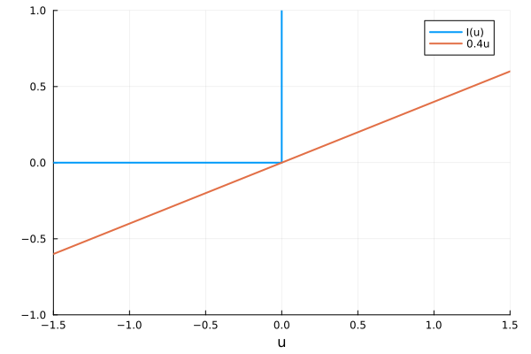
The Lagrangian relaxes the infinite step function

I(u)

to a linear penalty

\lambda u

with

\lambda\geq0

The polynomial sum-of-squares dual generalizes the Lagrangian to a polynomial dual, but not in the $u$ dimension. That is, the polynomial dual remains linear in the constraint ( $u$ ), but allows the dual to vary with the decision variable $x$ , so long as it is a sum-of-squares polynomial. We write $J_\kappa(x, u) = p(x) u$ for $p(x)\succeq_{sos} 0$ ( $p$ is a sum-of-squares). To visualize this, we need a third axis:

The polynomial dual (green) is still a linear function of the constraint

u

, but it allows the slope to vary polynomially with

x

Intuitively, varying the linear penalty term with $x$ is complements the constraint's variations in $x$ to give a better lower bound. Computing this dual and showing it is a convex program is fleshed out later in this post. Before we get there, a side-by-side comparison:

The Lagrangian dual is:

\begin{aligned} d^\star = \max_{\lambda\geq0}\ &f(0) + \sum_{i=1}^N \lambda_i g_i(0)\\ \mathrm{s.t.}\:& \hat f(x) + \sum_{i=1}^N \lambda_i \hat g_i(x) \succeq_{sos} 0. \end{aligned}

The polynomial dual from moment-sum-of-squares is:

\begin{aligned} d_\kappa^\star = \max_{\lambda_i \in \mathbb{R}_\kappa[x],\ \lambda_i(x) \succeq_{sos} 0}\ & f(0) + \sum_{i=1}^N \lambda_i(0) g_i(0)\\ \mathrm{s.t.}\:& \hat f(x) + \sum_{i=1}^N \hat \lambda_i(x) \hat g_i(x) \succeq_{sos} 0. \end{aligned}

I'm using a compact SOS notation, but this is the standard Lagrangian dual and moment-sos-hierarchy of order $\kappa$ . The key difference is the scalar dual variable $\lambda_i$ is replaced with a dual polynomial $\lambda_i(x)$ (of order $\kappa$ ). Both dual problems are convex, and the polynomial dual is guaranteed (under some regularity) to return the primal solution as $\kappa\rightarrow\infty$ . Let's explore these in more detail.

Lagrangian dual

In this section, we show the Lagrangian dual gives a lower bound to (1) and imposes a linear penalty on constraint violation. Eq. (1) is equivalent to:

p^\star = \min_x \max_{\lambda \in \mathbb{R}^N_{\geq 0}} f(x) + \sum_{i=1}^N \lambda_i g_i(x).

The new objective is called the Lagrangian. To see the equivalence with (1), consider the minimum and maximum together. If any of the constraints on $x$ are not satisfied, the maximum gives $+\infty$ which cannot be minimized. Thus, any finite solution requires all constraints to be satisfied. When all $g_i(x) \leq 0$ , the inner maximization is solved for $\lambda_i \equiv 0$ , yielding exactly (1).

The Lagrangian dual simply swaps the minimum and maximum. That is,

d^\star = \max_{\lambda \in \mathbb{R}^N_{\geq 0}} \min_x f(x) + \sum_{i=1}^N \lambda_i g_i(x).

Why is this dual useful? It's a concave program! The inner optimization problem is concave (more precisely, linear) in $\lambda_i$ . And the pointwise minimum (over all points $x$ ) of concave functions is concave (though it may no longer be linear). We'll make this precise in the next section. Taking the maximum of a concave function lies in the regime of convex optimization.

Importantly, the dual also provides a lower bound on the solution to (1). Consider the Lagrangian:

\mathcal{L}(x, \lambda) \triangleq f(x) + \sum_{i=1}^N \lambda_i g_i(x).

For any primal feasible $x$ (satisfying all inequality constraints) and dual feasible $\lambda \geq 0$ , we have the following two inequalities:

\lambda_i g_i(x) \leq 0 \implies \mathcal{L}(x, \lambda) \leq f(x),

and

\min_x \mathcal{L}(x, \lambda) \leq \mathcal{L}(x, \lambda).

Putting these together, for all feasible $(x, \lambda)$ we have:

\min_x \mathcal{L}(x, \lambda) \leq \mathcal{L}(x, \lambda) \leq f(x).

By taking the maximum over $\lambda$ on the lefthand side and the primal optimal $x$ on the righthand side, we have shown weak dualty.

Theorem. (Weak duality) The Lagrangian dual lower bounds the primal:

d^\star \leq p^\star

Specializing to polynomials

Let's make the concavity of the dual a little more explicit in the case of polynomials. We first introduce a little notation:

Notation.

f\in\mathbb{R}_d[x]

means

f(x)

is a polynomial in

x

of degree at most

d

Every polynomial $f \in \mathbb{R}_d[x]$ can be written as $[x]_{\lceil d/2 \rceil}^T A [x]_{\lceil d/2 \rceil}$ for some symmetric matrix $A$ (not necessarily unique). We call this a quadratic form.

Notation. $[x]_{d}$ is the vector of monomials of degree at most $d$ . For $x\in\mathbb{R}^n$ ,

[x]_{d} \triangleq [1, x_1, ..., x_n, x_1^2, x_1x_2, ..., x_n^d]^T \in \mathbb{R}^{C(d+n,\ d)}.

This is called the monomial basis.

Using the quadratic form of $f,\ g_i\in\mathbb{R}_{2d}[x]$ , we rewrite the Lagrangian as below:

\mathcal{L}(x, \lambda) = [x]_d^T A [x]_d + \sum_{i=1}^N \lambda_i [x]_d^T B_i [x]_d.

Recall that the first element of the monomial basis $[x]_d$ is $1$ . To derive the dual it is helpful to separate out the constant terms:

\mathcal{L}(x, \lambda) = A_{1,1} + \sum_{i=1}^N \lambda_i (B_i)_{1,1} + [x]_d^T \hat A [x]_d + \sum_{i=1}^N \lambda_i [x]_d^T \hat B_i [x]_d,

where $\hat A$ and $\hat B_i$ set the $(1,1)$ term to $0$ to remove the constants. From (7), we first minimize the Lagrangian over $x$ . Using the trace trick, separate $x$ from $\lambda$ :

\min_x \mathcal{L}(x, \lambda) = A_{1,1} + \sum_{i=1}^N \lambda_i (B_i)_{1,1} + \min_x \left\langle \hat A + \sum_{i=1}^N \lambda_i \hat B_i, [x]_d [x]_d^T\right\rangle.

Since $[x]_d [x]_d^T\succeq 0$ , the remaining minimum reaches $-\infty$ if $\hat A + \sum_{i=1}^N \lambda_i \hat B_i$ has any negative eigenvalues. Thus, we have the Lagrangian dual:

\begin{aligned} d^\star = \max_{\lambda\geq0}\ & A_{1,1} + \sum_{i=1}^N \lambda_i (B_i)_{1,1}\\ \mathrm{s.t.}\:& \hat A + \sum_{i=1}^N \lambda_i \hat B_i \succeq 0. \end{aligned}

This is just a convex semidefinite program! We've completed the scalar Lagrangian relaxation of our original non-convex polynomial optimization problem. By weak duality, we have $d^\star \leq p^\star$ . In the case $d^\star < p^\star$ , can we get a tighter bound or solve (1) exactly? Yes, using higher-order duals from the moment-sum-of-squares hierarchy.

Better lower bounds via moment-sum-of-squares

I've mentioned several times that the moment-sum-of-squares hierarchy replaces the scalar dual variables $\lambda_i$ with polynomial duals. Let's make this explicit. Eq. (1) is equivalent to:

p^\star = \min_x \max_{\lambda_i \in \mathbb{R}_\kappa[x]_{\geq 0}} f(x) + \sum_{i=1}^N \lambda_i(x) g_i(x).

The proof is exactly the same as the Lagrangian dual, noting that the notation $\lambda_i(x) \geq 0$ (in fact, we can use a weaker condition that $\lambda_i$ is sum-of-squares, but we introduce this later). It is perhaps unsurprising that the moment-sum-of-squares dual simply swaps the minimum and maximum:

d^\star_\kappa = \max_{\lambda_i \in \mathbb{R}_\kappa[x]_{\geq 0}} \min_x f(x) + \sum_{i=1}^N \lambda_i(x) g_i(x).

The same reasoning as before gives $d^\star_\kappa \leq p^\star$ . The special case $\lambda_i \in \mathbb{R}_\geq 0$ (all higher order terms are $0$ ) gives $d^\star \leq d^\star_\kappa$ . That is, the moment-sum-of-squares dual is at least as good a lower bound as the Lagrangian dual.

Theorem. (Weak polynomial duality) The polynomial dual is an upper bound on the Lagrangian dual and a lower bound on the primal:

d^\star \leq d^\star_\kappa \leq p^\star

I want to give some intuition as to why a polynomial dual might perform better than a linear dual. Mathematically, the dual polynomial has more degrees of freedom to maximize over (this manifests as matrix comparison, which we will see below). But the idea of the Lagrangian is to move constraints into the objective with a large penalty. A polynomial dual is a much more expressive penalty than a scalar dual.

We next derive the exact form of the polynomial dual.

The polynomial dual

For positive polynomials $\lambda_i \in \mathbb{R}_{2\kappa}[x]_{\geq 0}$ , the polynomial Lagrangian is:

\mathcal{L}_\kappa(x,\lambda(x)) = f(x) + \sum_{i=1}^N \lambda_i(x) g_i(x).

Note the subscript $\kappa$ , which indexes the maximum order of the polynomial duals and gives rise to a relaxation hierarchy. As with the scalar Lagrangian, we'll rewrite each polynomial in quadratic form and pull out the constant parts. Start with the product $\lambda_i(x)g_i(x)$ , which is a polynomial of order at most $2d+2\kappa$ . Breezing through some algebra, we can represent $\lambda_i(x)g_i(x)$ as $[x]_{d+\kappa}^T C_i [x]_{d+\kappa}$ . In quadratic form, the Lagrangian is:

\mathcal{L}_\kappa(x,C) = [x]_d^T A [x]_d + \sum_{i=1}^N [x]_{d+\kappa}^T C_i [x]_{d+\kappa}.

Notice that we now have a $N$ dual matrices $C_i$ , which we use for ease of exposition. From here the derivation is nearly identical to the scalar Lagrangian dual. Next, separate the constant terms:

\mathcal{L}_\kappa(x,C) = A_{1,1} + \sum_{i=1}^N (C_i)_{1,1} + [x]_d^T \hat A [x]_d + \sum_{i=1}^N [x]_d^T \hat C_i [x]_d,

where the hatted matrices have their $(1,1)$ element as 0 (they are polynomials with no constant term). From (18), we take the inner minimization of the polynomial Lagrangian over $x$ . We'll use the same trace trick to separate the dual variables from $x$ :

\min_x \mathcal{L}_\kappa(x,C) = A_{1,1} + \sum_{i=1}^N (C_i)_{1,1} + \min_x \left\langle \begin{bmatrix} \hat A & 0 \\ 0 & 0 \end{bmatrix} + \sum_{i=1}^N \hat C_i, [x]_{d+\kappa} [x]_{d+\kappa}^T \right\rangle.

In eq. (22), we pad $\hat A$ with zeros to account for the expanded polynomial basis. Noting that $[x]_{d+\kappa} [x]_{d+\kappa}^T\succeq 0$ , we must take the inner product with a positive semidefinite matrix to get a finite minimum. This constraint gives the dual problem:

\begin{aligned} d_\kappa^\star = \max_{C_i}\ & A_{1,1} + \sum_{i=1}^N (C_i)_{1,1}\\ \mathrm{s.t.}\:& \begin{bmatrix} \hat A & 0 \\ 0 & 0 \end{bmatrix} + \sum_{i=1}^N \hat C_i \succeq 0. \end{aligned}

What happened here? We simply absorbed the dual polynomial into a higher-order polynomial (the ring of polynomials is closed under multiplication). After that, we used the same steps as the scalar Lagragian to derive a dual problem!

A simpler way to write the above problem uses sum-of-squares notation and the more restrictive constraint that $\lambda_i(x)$ are sum-of-squares (explained in the next section). For the sake of comparison with (16), the polynomial dual is:

\begin{aligned} d_\kappa^\star = \max_{\lambda_i(x) \in \mathbb{R}_\kappa[x]_{\succeq_{sos} 0}}\ & f(0) + \sum_{i=1}^N \lambda_i(0) g_i(0)\\ \mathrm{s.t.}\:& f(x) - f(0) + \sum_{i=1}^N (\lambda_i(x) g_i(x) - \lambda_i(0) g_i(0)) \succeq_{sos} 0. \end{aligned}

Hopefully I've convinced you that this hierarchy generalizes the Lagrangian dual using polynomial duals. We've also seen that the polynomial dual cannot give any worse of a lower bound than the Lagrangian dual. It turns out we can make a much stronger statement: under some regularity, the polynomial dual converges to the value of the (non-convex) primal as polynomial order tends towards infinity. To see this, we first need a little background in sum-of-squares programming.

Sum-of-squares background

A sum-of-squares (SOS) polynomial is simply a polynomial that can be written as the sum of the squares of other polynomials. We'll use a convenient result from Parrilo (2003) to connect SOS polynomials to positive semidefinite matrices.

Theorem. A polynomial

p(x)\in\mathbb{R}_{2d}[x]

is sum-of-squares if and only if there exists

A \succeq 0

such that

p(x) = [x]_d^T A [x_d]

. This can be checked with a semidefinite feasibility problem.

This representation motivates the following shorthand notation.

Notation. We write

p(x) \succeq_{sos} 0

to mean

p(x)

is sum-of-squares. That is,

p(x)

can be written as

p(x) = [x]_d^T A [x_d]

with

A \succeq 0

SOS polynomials are an important subset of the set of positive polynomials $p(x) \geq 0$ . Checking whether a polynomial is positive is an NP-hard problem, but checking if $p(x)$ is SOS only requires solving an SDP.

Fortunately, strictly positive polynomials may be represented in part with SOS polynomials. This result is called a positivestellensatz.

Theorem. (Putinar's Positivestellensatz) Let $\mathcal{K} \triangleq \{x : g_i(x) \leq 0 \ \forall\ i\}$ , where $g_i(x)$ are polynomials (a basic semialgebraic set). Assume $\mathcal{K}$ is compact. If $p(x) > 0$ for $x\in\mathcal{K}$ , then

p(x) = p_0(x) - \sum_{i=1}^N p_i(x) g_i(x),

where $p_i(x) \succeq_{sos} 0$ for $i=0,1,...,N$ .

Rearranging (25), Putinar equivalently states that there exist $p_i(x) \succeq_{sos} 0$ such that:

p(x) + \sum_{i=1}^N p_i(x) g_i(x) \succeq_{sos} 0.

Note that Putinar guarantees the existance of some polynomials $p_i(x)$ and does not specify order. In practice, we must restrict $p_i(x)$ to order $\kappa$ . This leads directly to a hierarchy of relaxations which use higher-order dual polynomials.

Convergence to primal

In this section we'll show the following result, due to Lasserre (2001).

Theorem. (Hierarchy convergence) The solution to the polynomial dual converges to the primal solution as relaxation order $\kappa\rightarrow\infty$ :

d^\star_\kappa \rightarrow p^\star \text{ as }\kappa\rightarrow\infty.

Putinar's positivestellensatz is the key to the proof. Define the constraint set $\mathcal{K} \triangleq \{x : g_i(x) \leq 0 \ \forall\ i\}$ . The primal (1) is equivalent to maximizing a lower bound on $f(x)$ :

\begin{aligned} p^\star = \max_c \ &c\\ \mathrm{s.t.}\ & f(x) - c \geq 0 \text{ for all } x\in\mathcal{K}. \end{aligned}

Let's relax the constraint $f(x) - c \geq 0$ to $f(x) - c > 0$ and replace it with a sum-of-squares inequality using Putinar. We get the relaxed problem:

\begin{aligned} d_\mathrm{putinar}^\star = \max_{c,\ \lambda_i(x)\succeq_{sos} 0} \ &c\\ \mathrm{s.t.}\ & f(x) - c + \sum_{i=1}^N \lambda_i(x)g_i(x) \succeq_{sos} 0. \end{aligned}

By the relaxation to a strict inequality, we have $d^\star_\mathrm{putinar} \leq p^\star$ .

As an aside, we now show (29) is equivalent to the polynomial dual (24) with no constraint on dual polynomial order $\kappa$ . The constant terms can be absorbed into $c$ as follows. The $(1,1)$ element of the SOS inequality constraint reads:

f(0) - c + \sum_{i=1}^N \lambda_i(0) g_i(0) \geq 0 \iff c \leq f(0) + \sum_{i=1}^N \lambda_i(0) g_i(0).

Meanwhile, the remaining SOS inequality does not include $c$ . Thus, we can replace $c$ with its upper bound without changing the optimization problem, arriving at:

\begin{aligned} d_\mathrm{putinar}^\star = \max_{\lambda_i(x) \succeq_{sos} 0}\ & f(0) + \sum_{i=1}^N \lambda_i(0) g_i(0)\\ \mathrm{s.t.}\:& f(x) - f(0) + \sum_{i=1}^N (\lambda_i(x) g_i(x) - \lambda_i(0) g_i(0)) \succeq_{sos} 0. \end{aligned}

Having established equivalence, we now use (29) to prove the polynomial hierarchy converges. From duality, it holds $d^\star_\mathrm{putinar} \leq p^\star$ . Our strategy is to squeeze the dual with a lower bound. Let $x^\star$ solve the primal (1) with value $p^\star = f(x^\star)$ . Perturb $x^\star$ to $z=x^\star + \epsilon\in\mathcal{K}$ such that $f(z) = p^\star - \delta$ . The perturbed point $z$ enjoys strict positivity: $f(z) - p^\star > 0$ . Therefore, $z$ is feasible for the Putinar dual (29). Thus,

p^\star - \delta \leq d^\star_\mathrm{putinar} \leq p^\star.

Since $f$ is a polynomial we can make $\delta$ arbitrarily small by appropriate choice of $\epsilon$ . This shows that with arbitrary high polynomial order the polynomial dual converges to the true value and completes the proof.

The hierarchy convergence theorem is a remarkable result because it uses convex optimization techniques to solve a non-convex problem. It's worth pointing out, however, that there's no free lunch. Stepping up the relaxation order increases the size of the problem polynomially, making high-order relaxations essentially impratical in real-world applications.

Conclusion

That was quite a journey! Duality is one of the most interesting and useful concepts in optimization, and I find it remarkable that duality can be "generalized" for a class of otherwise hard polynomial problems. The bonus of a lower bound is the possibility of a optimality gap. Given a primal feasible point $x$ , the optimality gap is the difference between $f(x)$ and the dual $d^\star$ . There many rounding schemes to obtain a good guess for $x$ from the dual solution, and this metric is the main "certificate" in certifiable optimization research.

This line of reasoning led me to a few questions for further thought:

Is there a generalization of the dual for other classes of problems?
- Answer (probably): we need the dual to be convex in order to get good approximations. This greatly restricts the class of possible dual functions. Polynomials worked in this case largely because polynomials are closed under multiplication.
On the more practical side: are there other polynomial bases which have computational benefits?